Exploration Risks and Decisions – Part 4:
Valuing exploration optionality with risk neutral probabilities
This is part 4 of 6 in the series of articles that I will be publishing on the subject of exploration risk. Each part references subjects from previous posts and so should be read sequentially. The topics that will be covered are:
- Part 1: The sources of risk and odds of success in exploration
- Part 2: The optionality of exploration
- Part 3: Quantifying reserve volatility
- Part 4: Valuing exploration optionality with risk neutral probabilities
- Part 5: A statistically based Monte Carlo Model for exploration
- Part 6: Conclusions and implications for exploration participants
Introduction
The previous articles have reviewed exploration risk and how we may quantify it to incorporate into a real options model. We have broken down all the exploration risk factors into 2 volatility factors; commodity price and geological reserve or R. In the previous article we found a way to measure a reserve volatility Rσ, which is experienced through the exploration process as a discovery volatility Dσ. In this article we’ll look at one approach we can utilise to arrive at valuations for a given prospect. These valuations can also be used for management. The fundamental of exploration management is deciding when exploration spend is worthwhile, which requires a valuation of expected gains from exploration which this model can produce. In the next article we’ll look at an alternative improved model that utilises Monte Carlo Simulation.
Risk neutral probabilities
In earlier articles we have seen how exploration can be viewed in a real options framework. The techniques to value real options are intrinsically the same as for financial options. Risk Neutral Probabilities (RNP) was a technique developed in the financial world which we shall apply to our exploration real options model. Below is a brief description of the RNP method, a basic understanding of which is necessary for the model. Those of you with a background in option pricing may want to skip this section.
RNP explanation
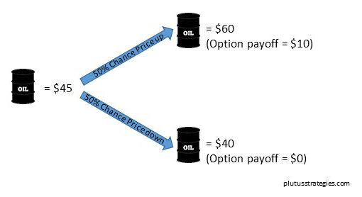
To explain how RNP works let’s use an example of a 1 year call option on a barrel of oil. The barrel itself is currently priced $45 but in a simplified scenario in one year it may be either $60 or $40. To exercise the option we must pay a $50 strike price, we shall assume a 0% interest rate. The real probability that the barrel of oil goes up $15 is 50% and down $5 50%. One approach would be that the option is simply the risked expected payoff and so the price is 0.5x10 + 0.5x0 = $5. This is incorrect as it assumes the market is risk neutral and indifferent to a definite $5 and an expected $5. In reality the market would demand a ‘risk premium’ and this is in evidence from the price of the barrel of oil in the first place, which is priced $5 below its expected return of; 0.5x60 + 0.5x40 = 50.
Oil Binomial Option:
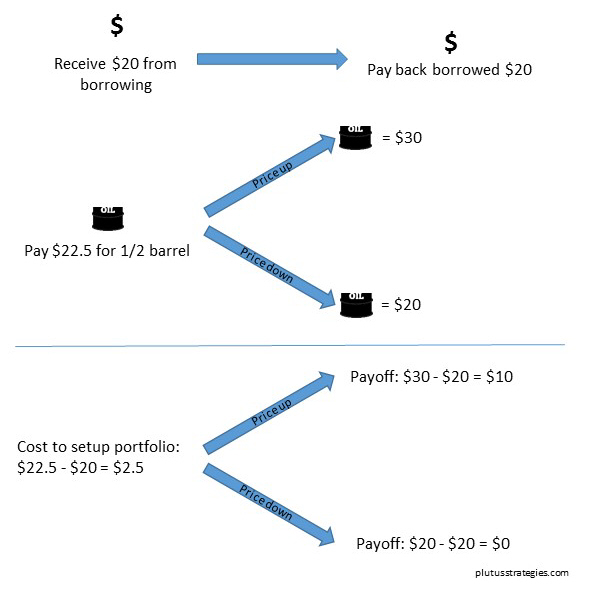
Another approach to price the option would be to create a ‘replicating portfolio’. This involves buying a fraction of the barrel of oil, and borrowing in such proportions that the outcomes at the end of the option period are the same as if you bought the option. If Δ is the fraction of a barrel of oil and B is the amount we borrow then 60Δ-B = 10 and 40Δ-B = 0, which solves to Δ=0.5 and B=20. Using the rule of no arbitrage (there are plenty of internet resources to explain no arbitrage theory for those interested), the price of the option must be the same as the price we pay to setup the replicating portfolio, $22.5 – $20 = $2.5. This is illustrated in the diagram below:
The Replicating Portfolio:
The important realisation is that we do not need to know anything about people’s risk preferences. As no knowledge of peoples risk preference is needed there is also no need to know anything about the real probabilities of the respective scenarios. The reason why no information is needed on the real probabilities or peoples risk preferences is needed is because all that information is already encapsulated in the price of oil in the first place.
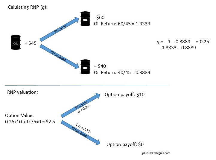
If we now imagine a different reality where everyone is risk neutral and only cares about expected return then the RNP (q) of the 2 different scenarios for buying the barrel of oil must be qx60 + (1-q)x40 = 45, which solves to q = 0.25. The underlying of both buying the barrel of oil and the option is the barrel of oil, so we can use this same RNP to calculate the option price; 0.25x10 + 0.75x0 = $2.5. This is the same answer as the replicating portfolio. The only measure we need to price a simple binomial option is the RNP q, it is not necessary to know anything about the real probabilities. The quickest way to calculate q is q = (r-ds) / (us-ds), where r = 1 + interest rate, ds = return on underlying in downward movement scenario and us = return on underlying in upward movement scenario. In this scenario q = (1 – 40/45) / (60/45 – 40/45) = 0.25.
RNP Model:
Exploration as a quadrinomial model
In the oil barrel example we imagined only one variable (price) and a binomial price up/down scenario. To model exploration we will need to accommodate both a price variable and resource/reserve variable which changes according to our discovery volatility Dσ explained in the previous article. This quadrinomial model for a gold prospect is illustrated below:
Exploration Quadrinomial Model:
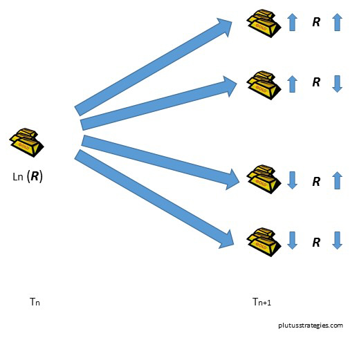
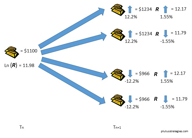
Let’s use the example of an Abitibi belt gold prospect we used in the previous article. Our initial gold price will be today’s spot price: $1100. The initial value for R is the natural log of the mean value from the distribution of R, described in the previous post and equal to 11.98. The respective up steps and down steps for R is determined by Dσ. For simplicity let’s calculate Dσ as Rσ spread evenly over the entire exploration lifecycle (for full explanation of Dσ and Rσ please read the previous article), this results in a value of Dσ = 1.55%. The gold price simply moves up or down according to the annualised standard deviation of the gold price which can be measured from historical price information, we shall use the value 12.2%. This process should be repeated for each node for the number of periods you wish to consider exploration over. I modelled this technique with my Abitibi gold example over 6 exploration periods which led me to arriving at 4096 (1 x 46) different project paths. Below is the first time period to illustrate the process, at the end of each node would be another 4 branch tree, ending in the 6th time period.
Quadrinomial Model of Gold Exploration:
The first step to valuation is to value the payoff at the end of each path by constructing simplified NPV models at each end node, based on assumed operating and capex costs. The costs should consist of a fixed component and a floating component, the rationale being that smaller resources tend to have higher costs per unit than their bigger brothers. An alternative may be to use a $/oz valuation with an added factor that depends on the gold price, exploration firms may find this particularly informative as these style valuations are easy to derive from comparable transaction analysis of deals at post feasibility stage. The valuation should never be less than 0 as there is no obligation to build an uneconomic mine.
After calculating the values at the end of each path, each individual node from right to left can be priced using RNP all the way to the starting point. The RNP’s for both the gold price and R can be calculated using the methodology given earlier. When calculating q for R the value for r (interest rate) should be 1, because R is not financial and doesn’t gain interest over time. These probabilities are multiplied together to give a combined RNP for each path of the quadrinomial tree. The outcome at the end of each branch is multiplied by the combined RNP, and all the branches are summed together to get the total value of all the outcomes. If the valuation at the node is greater than the cost of exploration then exploration proceeds, if lower, exploration is abandoned and the node is valued at 0. If exploration is deemed worthy, the true valuation is the sum value of all 4 branches minus the exploration cost for the next phase. Below is a diagram showing one of the 5th to 6th period branches.
Risk neutral pricing at T = 5:
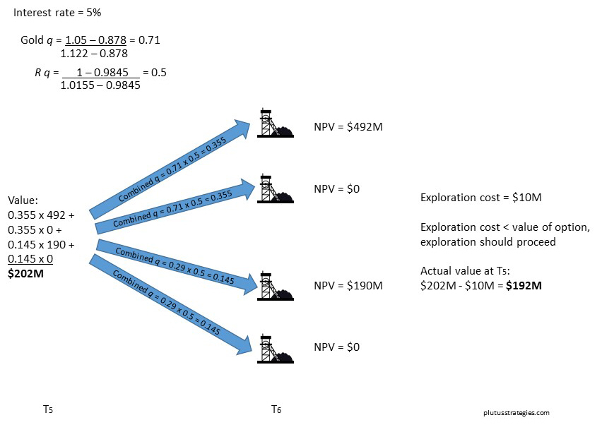
The values calculated at T=5 in the diagram above will form the values at the end of the branches in T=4, the calculated values at node T=4 will be the branch values for T=3, and so on until the model is priced back to T=0.
One of the advantages of this methodology is that you can quickly match a project to a corresponding node at the right stage of development and with similar values for R and price to derive a value. Exploration management can use these values to see if it is worth funding the next stage of exploration. Equally potential investors can identify the appropriate node to derive a valuation as the basis of an investment decision.
It is worthwhile pointing out here that the model assumes that the management will act rationally to stop unworthy exploration, and that cash is already within the company. If a further equity raising with shareholder dilution is required to complete the next stage of work (as is often the case) then this should be factored into the management’s decision.
Results of Model
At T=0 this model gives us the value of a grass roots gold prospect in the Abitibi belt, but without the conditionality that it will be successfully drilled d (see previous post). With today’s gold price the modelled value was $11.6M which is clearly too high given the market valuations of junior exploration companies at present, but this is without the conditionality d. We will look at d in a little more detail in the next post, but if we take some assumed values for success such as 20% chance of a prospect being drilled and 20% chance of that drilling being successful (i.e. will result in a mineral resource estimate of some description). We can apply the 20% x 20% = 4% success rate as a straightforward risk to our valuation, and the resulting value is $0.46M. This is a somewhat more realistic valuation but perhaps still a little high compared with current market valuations, bearing in mind that most junior exploration companies will have multiple prospects. Part of this discrepancy is no doubt due to peoples risk aversion as described in the RNP explanation. Note that the 4% odds of drilling success are real probabilities and not RNP, so we are comparing an expected $0.46M with a certain one. A significant risk premium should be taken into account and would result in a lower valuation.
When we constructed the model the up and down steps of R where calculated from the standard deviation of R. The standard deviation only encompasses 68% of expected values, and even if we were to bump it up to 2 standard deviations it would still only encompass 95% of values. This has significance as within the scenarios that lie outside of the standard deviation are the very rare ‘long tail’ scenarios of deposits of enormous size. Though these occurrences are rare they are an important motivation for people undertaking exploration and should really be accounted for in a valuation model.
This model clearly has its limits, it is perhaps most useful for managing exploration on projects that have already been successfully drilled. The property of being able to quickly identify a node that matches a given prospect and derive a value is a useful one. In the next post we will review an alternative model that utilises Monte Carlo simulation, a common valuation technique in the oil industry. The model will incorporate the conditionality d and we will use a more reasoned value of Dσ for each stage.