Exploration Risks and Decisions – Part 3:
Quantifying reserve volatility
This is part 3 of 6 in the series of articles that I will be publishing on the subject of exploration risk. Each part references subjects from previous posts and so should be read sequentially. The topics that will be covered are:
- Part 1: The sources of risk and odds of success in exploration
- Part 2: The optionality of exploration
- Part 3: Quantifying reserve volatility
- Part 4: Valuing exploration optionality with risk neutral probabilities
- Part 5: A statistically based Monte Carlo Model for exploration
- Part 6: Conclusions and implications for exploration participants
Introduction
In the previous posts I described how exploration on an individual prospect scale can be thought of in a Real Option framework as a compound option, and therefore can be valued and modelled using existing option theory. This model offers significant benefits over traditional techniques as it incorporates exploration risk and the value of the optionality of exploration which we know exist. One important component of the option model is volatility and we ended the last post with some of the difficulties in estimating volatility or σ of exploration projects. By volatility we are referring to a measure of the potential changes in prospectivity as exploration progresses. This volatility is a result of myriad risk factors which were summarised in the first article but at an early stage dominated by geological and technical risks. It is clear that there are many individual sources of volatility, each difficult to quantify, so that it would seem futile to try and ascribe a value to each. Furthermore, some factors would require some serious abstract thinking to apply the concept of volatility at all. This would present as an ideal point to draw on the work of previous workers in this field to find a way around the problem.
A single ‘R’ factor
Davis, G.A. and Samis, M. broke down the conundrum in a rather neat way in their 2006 SEG paper, which I urge interested readers to read. They made the reasonable assumption that ultimately the prospectivity, which is directly related to value, of an exploration project is derived from an ability to generate mineable mineralisation. Consequentially a projects value is a factor of the expected reserve base R multiplied by profit margin on each reserve unit; CAPEX can be considered separately and deducted as appropriate. Davis and Samis defined R as “… the quantity of mineralisation in a specific location that is of sufficient geological assurance and economic value to be profitably mined, either now or in the future, under currently forecast market and technical conditions”. The R factor represents only material that can be economically mined; therefore, it must include the various risk factors discussed in the first post (grade, metallurgy, geotechnics etc). It reminds us of reserves in respect of international reporting codes. However the major departure is that R does not need to be known with certainty. It is simply our best estimate of what might be minable at any time during the exploration process.
At earlier stages of exploration, no reserves are estimated, but when some drilling has taken place it is a common for a resource of some kind to be calculated. The Joint Ore Reserves Committee (JORC) defines resources as a solid material that occurs “…in such form, grade (or quality), and quantity that there are reasonable prospects for eventual economic extraction” and that they are converted into reserves upon the application of economic ‘modifying factors’. Resources are therefore roughly equivalent to R for early stage exploration prospects.
Resources, reserves and R
Many may baulk at the conflation of reserves and resources into a common R factor, and that is not without good reason. Resources are rarely converted 100% to reserves when more economic factors are considered. A 75% conversion rate is a rule of thumb that I have come across; and so for those who remain uneasy with a combined R, a conversion rate may be considered. Conversely resources that do not make it into a reserve at initiation of mining, often do get mined eventually. It is indeed not unusual that over its lifetime a mine may produce more than the initial reserve and resource estimates combined.
Another possible source of concern is that small resources may never become reserves as they never reach a threshold whereby reserves can be booked (worth noting that using a strict JORC definition these probably should not have been booked as resources in the first place). We can compensate for such occurrences at a mining stage by utilising minimum thresholds, below which resources hold no more than a resale value. For those still concerned that resources may not adequately represent what is mineable in the future, it is worth bearing in mind that in the context of R, resources are conservative. This is because resources may not include undrilled portions of mineralisation whose presence and quantity is not known with certainty, but is strongly suspected. These portions should be part of our best estimate of what may be mineable.
In order to fully capture R, which is our expectation of what is mineable, we shall consider R to be the sum of all resources and reserves regardless of classification or standard (including historical resources not completed to JORC/43-101). For those familiar with Soviet classification systems, it is interesting to note the similarity between R and ‘P’ category prognostic reserves.
Real Options vs resource geology
It is perhaps an opportune moment to emphasise that our use of R is to derive a value for volatility over an entire terrane. Our relaxed approach to R, and the abuse and malpractice that unfortunately may arise during an individual resource/reserve estimation, should not have an overriding effect on our calculations on a terrane wide scale; as long as there is no systematic bias introduced. If we are to consider individual prospects that have been drilled, resulting in a substantial amount of data, then a great deal of consultation should be made with the technical staff and careful consideration given to what R is for the prospect. Practioners should be wary of relying on possibly poor quality resource estimates (even those with a 43-101/JORC stamp) when considering specific examples to ensure their assumptions about R are correct. It cannot be stressed enough that R is not an estimate of what is definitely present, which is within the realm of true resource geology and not within the scope of these posts. These posts are not intended as a guide to resource estimation.
Reserve volatility
If we can accept the simplified model of the single R factor, it is apparent that the only project volatility we need to derive aside from commodity price volatility is that of R or Rσ. How do we go about that? One solution I considered previously is to look at the volatility of publically listed exploration companies whose value is ultimately derived from resources/reserves. This approach is problematic as such companies often derive their value from more than one prospect. Also, intuitively we know that Rσ must be different between a prospect in a well-understood coal basin in the USA and a completely grass roots gold prospect on a new African frontier. Furthermore, stock prices are derived from the problematic traditional valuation techniques we discussed in part 2 and can experience wild fluctuations based on market sentiment, which often isn’t particularly rational.
Writing off the market value of exploration companies as a way of determinating Rσ leads us to consider, in more depth, what Rσ really is. The amount of reserves, the grade, the metallurgy and the geotechnical properties, all boil down to the geology under the ground. On the time scale of man, this geology doesn’t change; therefore, trying to measure the volatility through the lifecycle of an exploration project is rather absurd.
Instead of thinking of Rσ as the volatility of the reserve base through time, it should be thought of as the volatility of R from prospect to prospect. Obviously through the exploration cycle the amount of R attributable to a project changes, but this is actually the volatility of the process of discovery rather than any fundamental change of the geology. It is in fact the volatility of our expectation of R, which diminishes through time and the exploration process as we understand more and more about the subsurface geology; or what can be termed as the ‘discovery process’. Our volatility for an individual prospect through the exploration cycle is a combined volatility of what actually exists Rσ and Dσ (discovery volatility).
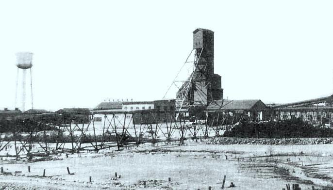
The Abitibi belt - a real example of measuring Rσ
Accepting that the volatility is actually that of not only what’s in the ground but also our expectations gives us a useful framework to work within. In order to understand this, let's study a very mature exploration province: the Abitibi gold belt of Canada. This area has been explored for hundreds of years with discoveries ranging from a fleck of gold in an isolated quartz vein to multi-million ounce mines. I have compiled a database from various sources of all the regions' resources and reserves. Loosening the term resources to include those which were not estimated to an international standard, such that the figures conformed to R as described previously. Many of the smaller ‘resources’ measure only a few thousands of ounces and are historic in nature and based on traditional sectional techniques, possibly from few holes. I felt that this information is still useful as it indicates that some R is present. All resources and reserves for the same prospect were combined into the common R factor.
When the log values of R are graphed, they follow a normal distribution. This means that R follows a lognormal distribution. This doesn’t appear to be a fluke, because when compared with the geologically similar West Australian gold field, a similar lognormal distribution is produced. The data is for hard rock resources only and omits alluvial deposits/occurrences.
Distibution of R
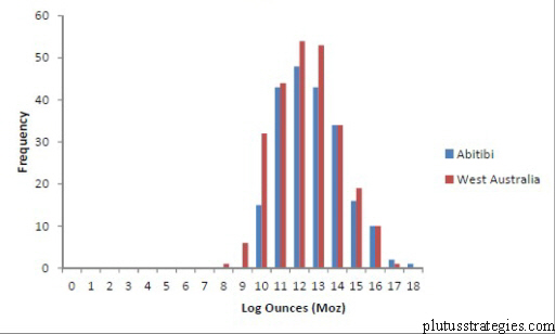
The lognormal distribution is a useful quality and the similarity between Abitibi/West Australia appears to show translation to other geologically similar but geographically separate terranes. The distribution only includes prospects for which resources have been calculated, and it is important to note that the majority of 1,000 mineral occurrences that we discussed in previous posts will never have any resources calculated. Many of the 1,000 are either determined unworthy of drilling or the initial drilling was unsuccessful. The distribution therefore allows us to model what may actually be present at any given prospect that is successfully drilled. The mean value of R (in this case 198,000oz) is our expectation at time 0 given the condition the prospect is successfully drilled. To keep our notation clear, let us represent the condition of successful initial drilling as d such that the mean value is d→R. If modelled over a number of prospects, this value will change according to d→Rσ. This is also the volatility of our expectations of R at time 0 at the beginning of exploration when we have no reliable exploration data to inform us of what R is. It is statistically represented as the standard deviation of R, which we can now accurately measure from the data. The condition of initial successful drilling d is important, and something we will return to in later articles, but for now it will suffice to just bear it in mind as a concept.
As an aside, it is useful to think in greater depth about this expected resource of 198,000 oz as calculated for the Abitibi belt. This figure falls below what most people in the industry would think would make a profitable, or at least financeable, conventional mine. Also this doesn’t even include the conditionality of d! Given the costs required to build and operate a 198,000 oz hard rock gold mine, it is likely to have an NPV deep in negative territory. Without flexibility, the prospect therefore has a negative value and exploration is seemingly never worthwhile in such a gold belt. However, exploration companies do exist and their very presence indicates that the market is already, to some degree, valuing optionality within exploration projects. They are thereby sub-consciously using an intuitive Real Options technique.
Discovery volatility
We discussed earlier what we observe as exploration progresses is actually discovery volatility Dσ. We can infer that Dσ over the entire exploration process must be equal to Rσ. This is because after feasibility everything should be known about the deposit and Dσ should be negligible. Unfortunately reality is often quite different but let’s stick with the theory for now! One approach to model Dσ is to break it down for each stage but ensuring that the overall volatility remains the same as Rσ. Intuitively we know that Dσ is higher at the earlier stages when less is known about the occurrence, so some qualitative interpretation may be required to appropriately distribute Dσ with extra weighting to earlier stage exploration.
Now that we have usable values for prospect volatility, we can combine this with commodity price volatility to have all the information we need to construct a meaningful Real Options based model for exploration. In my next post, we will construct a simple Real Options model based on risk neutral probabilities. In a further post, we will construct an improved model using Monte Carlo analysis, that incorporates the conditionality d and arrives at more reasoned values for Dσ.
References
Davis, G.A. and Samis, M. 2006. “Using Real Options to Value and Manage Exploration”. Society of Economic Geologists Special Publication 12, pp. 273-294.