
Exploration Risks and Decisions - Part 2:
The optionality of exploration
This is part 2 of 6 in the series of articles that I will be publishing on the subject of exploration risk. Each part references subjects from previous posts and so should be read sequentially. The topics that will be covered are:
- Part 1: The sources of risk and odds of success in exploration
- Part 2: The optionality of exploration
- Part 3: Quantifying reserve volatility
- Part 4: Valuing exploration optionality with risk neutral probabilities
- Part 5: A statistically based Monte Carlo Model for exploration
- Part 6: Conclusions and implications for exploration participants
Introduction
In my previous post I looked at some of the stages of the exploration process and the sources of risk inherent therein. We discussed how an understanding of the risks of each stage can lead to fair valuations necessary for both management to decide to proceed with exploration and for investors to estimate fair valuations in order to make investment decisions. The aim of this is to arrive at a model for exploration that tries to quantify the risks (and opportunities) presented by exploration, without relying on solely qualitative interpretation and handed down odds such as 1:1,000 success rates. Such a model can be a useful tool for both exploration management and investors alike. However before constructing a new model it may be helpful to look at some of the existing valuation techniques that are used.
Traditional Valuation
Exploration and mining projects are notoriously hard to value but let’s look at some commonly used methods.
NPV: It can be argued that the ultimate underlying value of an exploration project is the prospect of it generating a feasible mine which can in turn can be valued using conventional discounted cash flow analysis and Net Present Value (NPV). NPV is undoubtedly one of the most widely used and useful measures of value but does have deficiencies, in particular the method is inflexible and cannot accommodate changes in conditions or managements response to them. For example a very marginal mining project may have an NPV of zero implying the project has a value of $0. Intuitively we know this to be incorrect, particularly in low price environments, and that is because NPV cannot accommodate the optionality value of the project e.g. you may only decide to build the mine should the commodity price improve. Another drawback of the method is selection of discount rate which is often an arbitrary number that does not fully reflect the risk inherent in the project. NPV is often unsuitable for exploration projects where future cashflows cannot be predicted and it is this as well as the other deficiencies which have led to a number of other metrics to be applied:
- Book Value: Book value is the simple accounting value of the project and is the sum of all reasonable expenditure made on the project to date. This includes unproductive expenditures such as unsuccessful drilling.
- Appraised Value Method: The Appraised Value Method has some similarities to accounting ‘book value’, and defines the value of an exploration project to be directly related to the productive exploration expenditures to date and justified future exploration costs i.e. the cost of the next stage (but not stages after that) of work. The method requires a large degree of human judgement to decide which expenditures have been productive and can therefore produce widely varying values and is also therefore open to abuse by unscrupulous agents. Fundamentally the method does not value prospectivity so that 2 projects where expenditure has been the same but one has drilled stellar intersections compared to the others run of the mill intersections will be valued the same, this cannot be correct. Also problematic is that it may not reflect moves in commodity prices which we know to profoundly affect project value.
- ‘In the ground’ valuations: An industry favourite is ‘Dollar per Oz/t/lb’ style valuations whereby the weight of a commodity is given a value ‘in the ground’. The value in the ground is changed according to factors such as accuracy of measurement (inferred/indicated/measured), location, likelihood of mining and grade. Again a large amount of human judgement is required which can result in widely divergent valuations and leave the techniques open to abuse. It does however offer some improvement on the previous methods by reflecting prospectivity in some way and via comparable transaction analysis can provide a neat way for valuation during corporate deals.
Real Option Valuation:
None of the traditional valuation methods fully quantify exploration risk which is an essential component of an exploration prospects value. One method that can accommodate this risk is Real Options, a method that commonly finds application in other industrial and commercial projects. There is a plethora of helpful information sources on Real Options in general so I shall not go into any great detail of Real Options Theory save to say that most industrial and commercial projects can be thought of as an option to acquire some future economic value through either the establishment of cashflows or a capital gain. In its most raw sense the buying a mining project can be thought of buying the right to get a series of cashflows from mining, processing and selling ore. The right to build the mine does not have to be exercised and a company may only choose to do so if some fundamental such as commodity price improves. This is very similar to a financial call option on a mining company whereby we have the right to acquire an underlying mining stock which gets some financial reward from a mining project(s) but we are not obligated to acquire and may only choose to if the prospects of the mining project(s) improves (e.g. from a commodity price rise), and thereby the stock price exceeds the strike price.
The usefulness of this analogy is that all the risk of a financial option is encompassed in the price which can be accurately ascertained, if we apply the same techniques to Real Options we are able to accurately value projects with a consideration of the risk associated with them. A common tool for pricing European options (that is options with a fixed term with exercise only possible at the end) is the Black Scholes formula, this is a complicated Stochastic Differential Equation but if you don’t have a mind for maths don’t worry as a deep understanding is not essential. However for those of you interested I’ve included a brief intuitive explanation as a footnote to this article. Regardless of a deep understanding of the formula it is useful to look at the input parameters, how they compare to the real options world and the effect they have on option price:
Option Input Parameters
| Financial Option Parameter | Real Option Parameter | Effect of Increase on Option Value C | |
|---|---|---|---|
| S | Price of underlying stock | NPV of project without flexibility | + |
| K | Strike (exercise) price | CAPEX | - |
| r | Risk free rate | Risk free rate | + |
| τ | Option duration | Option duration | + |
| σ | Stock volatility | Volatility of underlying project | + |
| C | (Call) Option Price | Real Options value of project | n/a |
As a further explanation to the chart above as it relates to Real Options; S is simply the NPV of the mining project at acquisition, and can be thought of as someone acquiring the project with a firm commitment to begin mine construction immediately and thereby remove any optionality value. The volatility σ of a mining project is how much the value of the project S or the NPV may change over time. If we assume the project has an accurate feasibility study then changes in geological and technical factors should be negligible (in theory at least!) and the volatility is basically the volatility of the commodity price, with some additional volatility arising from changing inputs to capex and opex i.e. changing fuel or steel price. C is the call option price and in the example of the mine the Real Options value of the mining project. In practice a mining project is typically bought by a major off a junior and C can be thought of the money the major should pay the junior. The aim of the major should be to pay less to the junior than what it calculates the value of the project C to be, whereas the Junior should be negotiating for the full value of C.
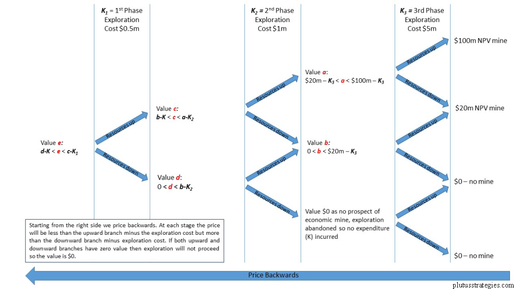
So a mine can be viewed as an option but can an exploration project? Exploration projects are more complex in that there are multiple opportunities to decide to halt exploration and walk away or carry on with the next stage so they are in fact a whole series of options or what is referred to as a ‘compound option’. In a compound option the underlying S is itself an option. This can be hard to think about for exploration, but if you could imagine an exploration project whereby the next step of exploration is to test the target with trenching, and the stage after is to conduct a scout drilling programme. The underlying option of the first trenching option is the option to scout drill. So that the S for the first option is the value of having the right to do scout drilling without conducting any trenching first. This may not be worth that much, as the chances are nothing will be found but should be above zero as there is no obligation to drill either. The value of S will change over time as we learn more about what lies beneath. If we begin to prove that mineralisation is not present S may dip below its original value as the right to conduct exploration or build a mine somewhere where there might be economic mineralisation is worth more than somewhere where there definitely isn’t economic mineralisation! S can also be thought of as the present value of project as calculated by one of the problematic traditional methods as described at the start of the post. It is obvious that S is rather hard to measure accurately for an early stage exploration project, fortunately this is not a problem as compound options are priced backwards from the end option which in the context of mining is the NPV of a theoretical mining project which with a few basic assumptions we can work out, this is illustrated in the diagram below:
Exploration as a compound option
So what of the other parameters of an option? Risk free rate is the same as for a financial option, for those of you without a financial background this is the annualised rate of return you can get from some riskless investment made over the same period. Traditionally the analogue has been the return you get from US government treasury bills, some of you may have your own opinions on whether these are truly riskless though! τ refers to duration and is the time it will take to arrive at the next decision point i.e. the time to undertake the next field season. C is the value of the prospect and ultimately what we are trying to discover, when acquiring a new prospect(s) management should ensure there calculated value of C is less than the acquisition price or they are overpaying.
Volatility (σ) is the volatility of the underlying option value i.e. the volatility of the prospects value. At first approach this may seem rather abstract when thinking about an exploration prospects but it is in fact the same ‘risk’ factors I talked about in the first post (if you haven’t read the first post I recommend you do so: Part 1: The sources of risk and odds of success in exploration). These risks create the volatility we see in the value of a prospect whereby as exploration progresses and we discover more about the various factors such as resource size or geotechnics the value of the prospect changes. This can be thought of as an all-encompassing change in ‘prospectivity’ that also includes a number of other geological factors that come in to play such as metallurgy, continuity, mining method etc. In this way a prospect that has drilled 10 holes with long intersections of sky high grades is of a higher value and prospectivity than an equivalent project with 10 holes with moderate intersections at run of the mill grade. In addition to the geological factors the prospect is also given volatility through fluctuations in commodity price. Fortunately this volatility can be accurately measured by looking at historic price behaviour. However the geological risk factors are seemingly impossible to assess in terms of volatility and are a crucial aspect in modelling exploration as an option. As it is such a crucial element I shall dedicate all of my next post to the subject.
As I mentioned earlier exploration is essentially a compound option where the underlying is another option, so for exploration the first phase of exploration gives you the right, but not the obligation, to conduct the second phase of exploration. This is where we can introduce the final parameter of the option, strike price K, as for to enact the second phase of exploration we need to pay the exploration cost and this is our strike price K. In other words our second phase of exploration does not derive its full value unless we are willing to initiate it by paying for more exploration, this is therefore the ’strike price’ we pay after a successful preceding phase of exploration. Another way to think about is that by paying K for exploration to occur we are releasing the volatility of the prospect by making it more or less prospective. Unlike the other parameters when K increases, it lowers C, the value of the option. There is some geological intuition to this. If we imagine 2 equally prospective grass root prospects but one is at surface and the other obscured by 25m of sand then the surface prospect is worth more as the amount of money we need to explore it K is less than for the sand covered prospect.
The utility of the compound option model
So it can be seen that the necessary correlations between exploration and financial options exist for us to utilise option theory to value prospects. This has important implications for management, for if the value of the option at any stage is lower than the exploration (strike) price needed to enact the option then it should not proceed and the prospect abandoned thereby ensuring capital is deployed optimally. For the investor the implication is equally straightforward, the ultimate value of an exploration company is an aggregate value of their various prospects, plus cash in the bank minus the cost of their next phase of work. Often each phase of work would signal a new financing round and for an investor participating in that round the crucial question they must answer is the market cap of the company under or overvalued compared to the modelled value C? As exploration finance is predominantly equity based they also need to factor in further dilution from future financing rounds.
In the first article I explained that the preeminent source of risk in exploration is geological and technical and in this article that this equates to prospect volatility which is the subject of the next article where we will look at ways we may estimate this essential component of the future model.
Footnote: The Black Scholes formula
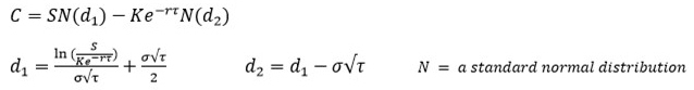
For some basic intuition of the formula without getting bogged down in calculus I find the following way of thinking of the formula helpful. The first half is SN(d1), S is the price of the company’s equity which is determined by peoples risk neutral future expectations of what may happen to the company, it is useful to think that it is the discounted equity value of all possible future states weighted by the chance of that state happening. S is then multiplied by N(d1) which is a measure of how much the value of S is composed of states that would result in option exercise, in other words the values of all the different future states where S would be greater than the strike price weighted by the probability of that state occurring. N(d1) can be thought of as a measure of how sensitive the option is to price movements. The second half of the formula –Ke–rtN(d2) is the discounted value of the exercise price Ke–rt multiplied by the chance that exercise will happen N(d2).